“Hey, Vince, when will the aurora be out?”
It’s the question I get the most on social media, and now, instead of saying… “well, it’s complicated…” I can point them to this blog post! So, when will the aurora be out? Let me tell you!
First off, I highly suggest you first watch my presentation at the 2023 Aurora Summit that goes over this entire topic starting with what is space weather and ending with the best resources for tracking the aurora. It really is a comprehensive guide from "Sun to Mud” that’s squarely aimed at beginners and should be relatively easy to understand regardless what skill level you are. But as I said at my talk at The Aurora Summit, there is no way to explain all of space weather and auroras in one presentation or blog post. As such, this guide is just meant to wet your appetite (and it's still over 20 pages long - yeah, aurora forecasting is complicated) for space weather science but also give you actionable items that you can take into your aurora chasing routine!
I even have the slides publicly available here with clickable links here!
With that out of the way, let’s begin!
Everything related to the aurora starts with the Sun - it’s what powers almost every process here on Earth. The conditions around the Sun and in space are always changing, and just like we have weather here on the ground, up in space, we also have weather - space weather! There are four main types of space weather that can affect our modern technology and infrastructure: high speed streams (HSSs), coronal mass ejections (CMEs), radiation storms, and solar flares. For this post, I will not be explaining radiation storms since they have no bearing on the aurora.
If you’re looking for a broad but succinct overview on these space weather phenomena, I invite you to read my peer-reviewed publication: “How open data and interdisciplinary collaboration improve our understanding of space weather: A risk and resiliency perspective.” It’s a bit sciency-sounding and the text is aimed at subject matter experts, but if you’re interested in how space weather can affect our ground- and space- based assets on and around Earth, then it’s a good read!
Now, before we delve into space weather - high speed streams, coronal mass ejections, and solar flares - we need to talk about the solar wind for some important context.
The Solar Wind
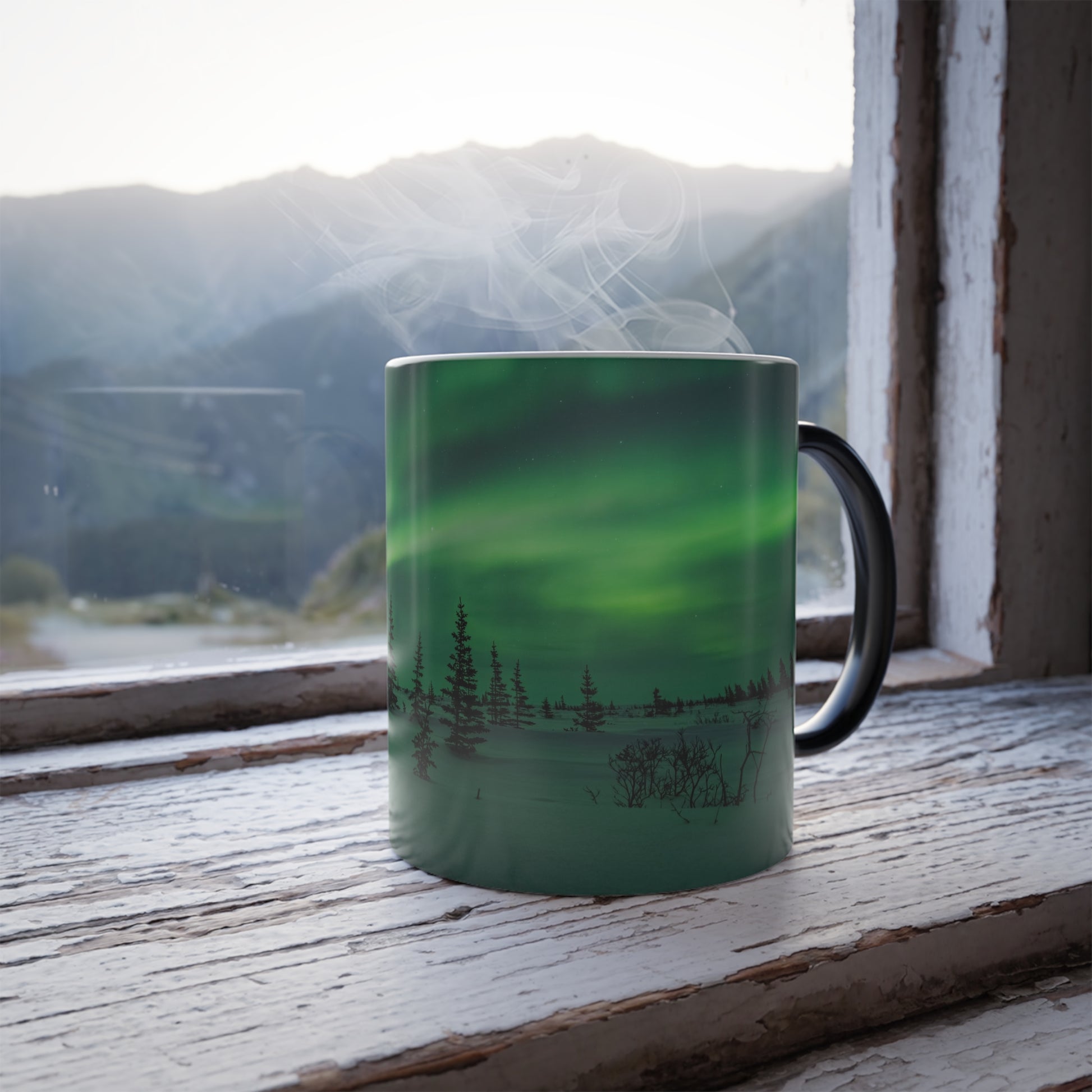
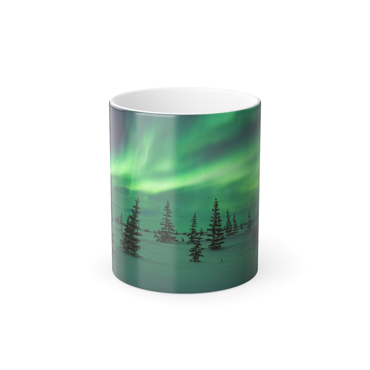
Imagine the Sun as a hot cup of coffee (maybe in one of my aurora magic mugs? - shameless plug, I know). Naturally, steam will form off the hot cup and waft into the air, and much like a hot cup of coffee radiating steam, the Sun is a hot ball of gas and plasma emitting a constant stream of charged particles into outer space called the solar wind. Unlike a hot cup of coffee, though, solar wind is not steam, and instead is a tenuous stream of electrons and protons that carry with them a magnetic field. This solar wind pervades the solar system and its pressure keeps all the planets within a sort of bubble that we called the heliosphere. The Sun also rotates, on average once every 27 days, and because of this rotation, the magnetic field threaded through the solar wind actually forms a sort of ballerina skirt that we call the “Parker Spiral,” named after the renowned solar physicist Eugene Parker.
Here is a helpful NASA video showing the effects of the solar wind.
Earth has a magnetic shield called a magnetosphere. The magnetosphere carries with it Earth’s magnetic field that is generated by the dynamo deep inside the core. When solar wind impacts our magnetosphere, depending on the orientation of the magnetic field in the solar wind, its energy can either penetrate into Earth or be deflected back out into space. The solar wind is what carries the energy that eventually causes the aurora.

High Speed Streams
The solar wind normally flows out from the Sun at around 300-400 km/s. While that’s already fast, in high speed streams, the solar wind can reach speeds upwards of 800 km/s! The convention is that speeds above 400 km/s are considered "fast" in the solar wind. Faster solar wind means there is more energy (more “oomph”) behind the charged particles, and when those particles hit Earth, they cause more impact. These high speed wind streams originate from areas on the Sun known as “coronal holes.” No, there are not physical holes, but if we take pictures of the Sun in shorter wavelengths than we can see, in the extreme ultraviolet (EUV), cooler regions appear darker, and when you have a large dark blotch on the surface, that’s what we call a coronal hole.
Here is a video showing a coronal hole rotating on the Sun captured by NASA's Solar Dynamics Observatory (SDO) AIA instrument.
The actual physics going on is not too complicated - the Sun has magnetic fields all along its surface, some looping across in arches and some flowing directly out into space. The looping or closed magnetic field lines trap particles and cause them to heat up. Regions of closed magnetic fields then appear brighter in EUV since those areas are hot. Open magnetic field lines, on the other hand, allow particles to freely flow away from the Sun out into space. These areas appear darker in EUV imagery and are called coronal holes.


Images of a coronal hole taken by SkyLab. This particular coronal hole persisted on the Sun for six solar rotations (almost six months). Credit: stanford.edu
The National Oceanographic and Atmospheric Administration’s (NOAA) Space Weather Prediction Center (SWPC) includes the possibility of recurrent high speed streams in their 27-day forecast. Basically what this means is if we experienced a high speed steam, NOAA assumes we will be impacted by the same fast wind from the same coronal hole 27 days later. Of course, coronal holes don’t last forever, they eventually close up and disappear, so these 27-day forecasts should be taken with a grain of salt.
Identifying coronal holes using real time solar wind is relatively easy - look for a slow density ramp that tapers off at the same time as a speed ramp occurs. This is indicative of the fast solar wind forcing slow wind ahead of it into a compression region. Fast solar wind streams also typically have hot electron temperatures. CMEs typically have cooler electron temperatures. I will be releasing a full tutorial on how to read solar wind soon, so I won’t delve too much into it here. But enough about coronal holes, let’s get to the “fun” space weather phenomena (at least in my opinion). Let’s talk about solar flares!

Solar Flares
Solar flares are like paparazzi flashes going off on the Sun - intense bursts of electromagnetic radiation that look like flashbangs in EUV imagery. While the light of the Sun is quite intense in the visible spectrum and overwhelmes the light of solar flares, very powerful events can sometimes be seen in “white light” (science talk for the light we see in the visible spectrum). The first direct observation of a solar flare was the one responsible for the Carrington Event in 1859, seen directly through a telescope here on Earth. Most notably, the solar flare preceded an intense geomagnetic storm that occurred 17 hours later, causing widespread auroras around the world. While it wasn’t known at the time, what happened was that the solar flare launched a very fast coronal mass ejection that slammed into Earth causing one of the biggest geomagnetic storms in recorded history. The solar flare itself did nothing…
Solar flares do not cause aurora directly. They are merely big flashes of light. Since they are only light, we see them as they happen - there is currently no way to predict when a solar flare may occur. Instead, we have detectors in space that tell us when flares happen. The most notable instrument is the GOES X-RAY detector, and flares are seen as sharp spikes in the graph. They are recorded on a logarithmic scale (like decibels for sound or the richter scale for earthquakes) and go from A (weakest), to B, C, M, and finally X (strongest). Anything above a C flare is noteworthy. A and B flares are not important.

Top: The GOES x-ray flux showing numerous solar flares, credit: spacewather.com.
Bottom: NASA video explaining the differences between solar flares and CMEs.
So why do we care about solar flares if they don’t cause aurora? Solar flares can launch coronal mass ejections out into space - physical matter, not light - which if directed at Earth, can cause geomagnetic storms when they impact. Let me reiterate that - solar flares, by themselves, do not cause auroras! This is a major misconception in aurora chasing communities that needs to be corrected.
Is there any way to tell what solar flares will launch CMEs? Yes. While it’s a bit beyond the scope of this blog, I will mention it briefly. Long duration flares or events (LDE) almost always are associated with CMEs. You can tell what flares are LDE because they have a slow decline down from flare peak to background levels. You can also examine EUV imagery and look for a blast wave from the source region where the flare occurred (called an EIT wave) or coronagraph images and look for a CME there. I’ll cover some of these resources later in the blog.

Coronal Mass Ejections
Coronal mass ejections (CMEs) are like “sun sneezes” - ejections of plasma away from the Sun out into space. These CMEs carry with them their own magnetic field like a bubble, but ride along the solar wind. CMEs can be launched by solar flares from active regions or can spontaneously lift off from the solar surface from filaments or prominences.
A spectacular CME as seen by SDO/AIA.
Since they can be launched in any direction from the Sun, sometimes they are directed at Earth and sometimes not. This makes modeling their trajectory through the solar system very important and also crucial for determining their arrival time at Earth (if they are directed at us). While HSSs can give us geomagnetic storms, their severity will usually cap out at a G2 (Kp 6) or G3 (Kp 7) level. CMEs can cause extreme space weather, and the biggest geomagnetic storms have all been from CMEs. This also means they can cause the best auroral displays. HSSs are easy to track, however, and we can see them many days before they affect us - high speed solar wind at the center of the solar disk will reach us in about three days. CMEs on the other hand can’t be predicted, but unlike solar flares which just emit radiation at the speed of light, CMEs take anywhere from 1-4 days to reach us. So once a CME is seen lifting off the Sun, you still have time to charge your batteries and make plans to chase the aurora.
Let’s talk about tracking space weather - how do you know when to expect enhanced activity and the best chances of beautiful auroral displays?
Tracking and Predicting Space Weather
Tracking and predicting space weather is tough. Nailing the arrival time of a CME heading towards Earth is like predicting how much snow a storm will give you if that storm was in two weeks. Many scientists have said “space weather forecasting is where terrestrial weather forecasting was in the 1960s.” There are just not enough data points to construct an accurate picture of what is going on from the Sun to the Earth - all we have are a few satellites monitoring the Sun and nothing in-between. When we see something happen 93 million miles (150 million km) away on the solar surface, it’s up to the models and our best judgment to say what if any affects there will be at Earth. Basically, what I’m trying to say is while forecasting space weather is possible, it’s hard, and there is never certainty. That being said, space weather forecasting is still useful and can give us insight into what may be coming our way. Let’s dive in.
High Speed Streams
High speed streams are easy to track - since they emit from coronal holes, which are easily visible in EUV imagery, we can get an idea of where the fast solar wind is by monitoring the position, size, and intensity of the coronal hole as it rotates with the Sun. The center of the solar disk as seen by Earth, often called the “Earth strike zone” is where anything from the Sun will be flowing directly at Earth. As such, when the coronal hole is at the center of the visible disk is when the high speed stream is likely 2-3 days away. The time lag is due to the fact that the solar wind takes time to get to us. So when we actually experience the fast solar wind, the coronal hole will be turning away.

The best way to see coronal holes is by looking at SDO EUV images, specifically the 211 or 193 Angstrom channel (21.1 or 19.3 nm). That filter really enhances color regions of plasma in the corona (coronal holes). Solar wind models like the WSA-ENLIL model also show high speed streams and the compression regions and can be used to predict when they will interact with Earth. Furthermore, NOAA SWPC will post a bulletin if a HSS is expected to become geoeffective. These brief news articles are also released for incoming CMEs once they have been modeled. HSSs show up on the 27-day Kp forecast, but like I said earlier, coronal holes may close up or become larger, either quenching or enhancing the high speed stream. These 27-day forecasts are not updated regularly and are not that reliable, so if a coronal hole changes shape, affecting the propagation of the high speed stream, the forecast won’t necessarily reflect that immediately. Use the 27-day forecast with caution!

SDO/AIA (193 Angstrom) showing a large southern-hemisphere coronal hole.
Solar Flares
There are currently no operational tools to predict solar flares. Since light travels at the speed of light, we see a solar flare as it’s happening. Flares can give us information on CMEs, though. If you see a LDE, a CME was launched with that event. Most strong (M-class and higher) solar flares are associated with some sort of mass ejection, and while tiny solar flares can cause large eruptions, the largest solar flares are usually associated with the fastest and most powerful CMEs. I recommend monitoring flare activity just to know the general state of the Sun - is it active or not - and watching for LDEs that can inform you when to look at other data sources to observe CMEs.
The best tool to track solar flares is the GOES X-Ray Flux.

Coronal Mass Ejections
Coronal mass ejections are big clouds of plasma ejected from the Sun out into interplanetary space. These blasts can be wide, narrow, slow, fast, symmetric, asymmetric, and highly structured. They are hard to track through space, and many operational models make assumptions to be run in real-time. To be honest, while you should always read NOAA SWPC’s predictions of CMEs since they are the official space weather forecasting office for the United States, it does not hurt to interpret the data and models for yourself! That’s the scientific process after all!
While NOAA SWPC is the official forecasting office, NASA does have their own space weather forecasting center in their Moon-to-Mars (M2M) office. NASA’s space weather operations focus on their missions in the heliosphere (e.g., Parker Solar Probe or the Mars rovers) and the Artemis programs. Both forecasting offices use the WSA-ENLIL model which I mentioned earlier. When a CME is launched from the Sun, NOAA and NASA will input parameters of the CME (mass, speed, angular width, etc.) into the ENLIL model and release a run for that event with an arrival time and impact speed and density. The NASA enlil model runs are put out a bit faster than NOAA models and are found on the NASA Coordinated Community Modeling Center (CCME) CME scoreboard site. Other scientists and forecasting offices can also submit their own CME models for specific events. Each CME is also cataloged on this site which is helpful when there are many events taking place per day as is the case now during solar maximum. Each event gets its own listing on the CCMC Scoreboard where model runs can be uploaded. Please note that while the CME scoreboard is a fantastic resource, it’s pretty experimental and not meant for operations. I do not recommend publishing model runs on social media and taking them as gospel. Just like a hurricane’s path might differ between three or four weather models, so does a CME’s path through space. Look at all the data, models, forecasts, and information and form your own opinion.


The ENLIL models will give you an impact time and estimated speed and density profile of the CME when it impacts. The accuracy of these impact times depends on a lot of factors. For example, if the CME is barely visible in imagery and has a weak signature, the model will likely not be as accurate as if the CME was strong and easily traced as it left the Sun. I find that the impact times are accurate within 7-12 hours of arrival, so don’t get upset if you convert the UTC time of impact and it ends up being for midday at your local time. It shouldn’t be taken that seriously.
How can you detect CMEs lifting off the Sun? In my talk I gave at the Aurora Summit, I go more into depth on this subject, and to be honest, it deserves an entire blog post, but CMEs can be seen in EUV imagery as well as coronagraphs. We know EUV images from SDO, but tools like SolarDemon apply a special filter that makes it easier to track changes in the Sun’s corona. This way, you can see blast waves coming off the Sun and get a sense of how far they propagate.

Coronagraphs create artificial eclipses of the Sun using an occulting arm so that images can be captured of the faint light scattered from dense structures in the solar wind. The LASCO C2 and C3 cameras onboard the SOHO spacecraft and the Cor2 camera onboard STEREO-A’s SECCHI instrument are the only coronagraphs currently in operation. CMEs are seen as little puffs of light off the occulting disc.

The SOHO spacecraft is positioned at L1 in between the Sun and the Earth, so if a CME is headed at us, you will see a halo of material propagating radially outward from the occulting disk. This is called a “Halo CME.” CMEs can also have “partial halos” that indicate some Earth-directed component. An automated CME-detection tool called CACTus is a nice resource to look at if the CME is not obvious in coronagraph imagery. Otherwise, just like SolarDemon applies a differencing filter to EUV images, SEEDS applies a differencing filter to LASCO C2 images, allowing faint CMEs (sometimes called stealth CMEs) to be more easily seen.

While I definitely have some experience with CME science and modeling, even I have to admit that it is hard to look at a coronagraph and determine whether a CME is Earth-directed and when it will arrive. Scientists with decades of experience might be able to, but I cannot, and I recommend defaulting to degreed subject matter experts for CME analysis.
How can you detect CME impacts? In real-time solar wind plots, CME impacts appear as shocks, or sharp rises in speed, density, and magnetic field. These shocks are also sometimes called “sudden impulses,” and if you are subscribed to the NOAA SWPC alerts, you can get text and email notifications when these impulses are detected.


Canonical solar wind profiles of CME impact (left) vs. coronal hole high speed stream (right). Below are actual data of these events seen in real time solar wind. Adapted from Kataoka et al. (2006).
A few hours leading up to impact, it is possible to sense the CME approaching Earth using the ACE satellite’s electron proton and alpha monitor (EPAM). The physics going on here can be simply explained, but the devil is in the details as always. When a CME is launched from the Sun, low energy electrons and protons are swept up by the shockwave and can be accelerated in front of the CME. If the CME is approaching Earth, you will see the density (particles per unit volume) increase steadily followed by a sharp ramp up right before the CME impacts as the shockwave passes over the ACE satellite. This is a good way to tell if a CME is close to Earth and since CME shocks can drive aurora immediately after reaching Earth, ACE EPAM can give you a few hours heads up before the show starts. The only caveat with ACE EPAM is that the low energy particles not only propagate in front of the CME but also to the sides, so it’s possible to see a ramp up in density of these low-energy particles without seeing the CME ever impact. Furthermore, if there are multiple CMEs in transit from the Sun to the Earth, it’s hard to tell when one CME signature ends and another starts. In other words, during solar maximum when there’s a lot of “junk” in space and ejections every day, relying on ACE EPAM can do more harm than good. Even still, it’s a good resource to use.

Space weather tracking “workflow”
Here’s what I recommend doing if you want to track a space weather event from the moment it occurs on the Sun to the moment it reaches us here on Earth. This applies to CMEs since HSSs can be seen days in advance and predicted with reasonable certainty.
- CMEs are often associated with solar flares. If a solar flare occurs, if it is LDE, then a CME was launched. Monitor GOES x-ray flux for flaring.
- Check CCMC CME Scoreboard for the latest model runs with arrival times. If it looks like a weak CME, then chances are the impact will be small and the arrival time may be only accurate within 12-24 hours. If the CME looks strong, chances are the arrival time is more accurate, maybe within 12 hours.
- If you want to do your own analysis, check SolarDemon and SEEDS to see the event unfold. Make your own predictions, but remember that accurate analysis of a CME’s trajectory through space takes years of experience and much more advanced knowledge than I can cover in a blog post.
- Check to see if NOAA has released their own ENLIL model. Usually, the M2M office is quicker than NOAA and SWPC takes their time. Sometimes this benefits in a better arrival time prediction.
- Close to the arrival time, check solar wind data from ACE and DSCOVR and look for the CME arrival in ACE EPAM. Look for “sudden impulse detected” notifications from NOAA SWPC.
- After impact, transition to aurora monitoring “mode.”
Tracking the aurora
Hopefully you are still following along, sorry this blog reads more like a book, but I want to be as complete about my information as possible, and nothing in space weather and aurora prediction is ever simple.
So far, we have talked about events on the Sun propagating out into space, into the solar system and throughout the heliosphere, but what happens when the solar wind and enhancements such as high speed streams or coronal mass ejections reach our planet? Do charged particles from the Sun directly hit our atmosphere and cause auroras? How are auroras actually created?
In space physics, we can break the entire Sun-to-Earth connection down into four domains. First is the Sun itself, its interior, surface, and atmosphere. Then, interplanetary space - the domain through which space weather travels. Then, we get to Earth and the magnetosphere, another regime. Finally, we get to the ionosphere and the ground, the final step from “Sun to Mud.”
The magnetosphere
We have already covered the first two domains, so let’s talk about the last two. The magnetosphere is a protective shield around our planet that deflects solar wind like an island in a stream of water. Earth is a giant bar magnet with field lines running from the south pole to the north pole. Fields, whether they are gravitational, magnetic, or fluid, are vectors with directions of propagation. If we define a system of directions where “x” is radial of the Sun, “y” is in the ecliptic plane, and “z” is perpendicular to “x” and “y,” we can describe different components of the magnetic field. The “north” direction of Earth’s magnetic field is actually a positive-z component for example. This will become important later.

The orientation of the x, y, and z components of the solar wind's magnetic field, credit: Space Weather Live.
Earth’s magnetosphere protects us from the solar wind and particles directly entering the near-Earth space environment, but there are ways energy from outside can enter. The solar wind also has a magnetic field associated with it, and if the z-component of the solar wind magnetic field is oriented in the south or negative direction, when it comes into contact with Earth’s north or positive-z magnetic field, a process known as magnetic reconnection can take place. This magnetic reconnection transfers energy from the solar wind’s magnetic field to the Earth’s magnetic field and particles can then flow freely through our “shield” down to the geomagnetic poles. This magnetic reconnection takes place on Earth’s dayside - the side of Earth facing the Sun because, obviously, the solar wind comes from the Sun, so it hits Earth’s dayside when it impacts us. When this magnetic reconnection happens, the energy that immediately funnels down to our geomagnetic poles creates dayside aurora known as “cusp” aurora. This is really only visible in Svalbard, and cusp aurora is very weak and faint, so it is only visible for a month around the winter solstice in December.
The two newly-formed magnetic field lines are now open out into space and get draped back over Earth’s magentosphere by the solar wind pushing them along. Eventually, the Earth’s magnetosphere pinches off in the magnetotail, and these two field lines reconnect again on the nightside, forming one new magnetic field line that sends its particles back to the geomagnetic poles again. This is called “nightside reconnection” in the magnetotail, and the entire process of reconnection on the dayside and nightside due to Bz-south solar wind is called the Dungee Cycle. This is a fundamental concept in how the solar wind couples with Earth and why as aurora chasers, we obsess over what the Bz is doing! Bz-south is like an “on” switch for the aurora, and the lower the Bz goes, the better (generally speaking).


What this means is that no, solar wind doesn’t stream out from the Sun and directly impact our planet - there is an entire process that governs how energy is transferred into Earth’s magnetic system and down into the aurora.
Beyond nightside reconnection, I am not going to get into other forms of aurora generation, but let it be known that nightside reconnection is not the entire story.
NASA animation of magnetic reconnection through the Dungey cycle.
The ionosphere
Once the particles get slingshotted back to Earth from magnetic reconnection, they eventually hit a region of our atmosphere called the ionosphere. The ionosphere actually separates into multiple layers that overlay the thermosphere (just a little technicality to point out), and auroras occur in the upper-most regions. When charged particles from the magnetosphere hit the ionosphere, they interact with gasses like nitrogen and oxygen in a process called ionization (part of why it’s called the “iono”-sphere, too) and emit light as a byproduct. The wavelength of light emitted corresponds to the gas being ionized and because the ionosphere is composed of different types of gasses at different heights, we get pink, green, and red aurora. The exact heights and colors produced are shown in the diagram below.

Behavior of the aurora
On a macro-scale, the auroras occur in oval rings around both geomagnetic poles. These are called the auroral ovals. Auroras in the northern hemisphere are called aurora borealis, and auroras in the southern hemisphere are called aurora australis. These ovals “breathe” with the intensity of the solar wind - more intense solar wind causes the ovals to expand and move towards the equator while less intense solar wind causes the ovals to recede to more northerly latitudes. On average, the auroral ovals are directly over 66-68o magnetic north. Places like Coldfoot, Alaska, Churchill, Manitoba, Tromso, Norway, and Akureyri, Iceland are all at these geomagnetic latitudes. In other words, they experience overhead auroras almost every night (weather permitting).
On average, 1-2 times per night, the aurora oval goes through a substorm cycle where it expands equatorward and forms dynamic structures (see the seminal Akasofu (1964) paper for more information). These substorms are initiated from a specific point along the oval then spread out across the globe, almost like throwing a stone in a lake and watching the ripples move outwards. Substorms are hard to predict, but I have an entire blog post on how you can use the GOES Magnetometers to better understand when they may happen.


Along with magnetic latitude and longitude, there is also magnetic local time. All these quantities are determined by your position relative to the magnetic north or south poles which are not at the same places as the geographic poles. In fact, the magnetic south pole is actually more offset than the magnetic north pole is from its geographic counterpart. Isn’t that odd!

As your point on Earth’s surface rotates from dusk to night (let’s say you are in Fairbanks, Alaska and conditions are quiet), you will see the auroral oval move equatorward and the aurora starting in the northeast moving more due north and slightly overhead. When the auroral oval is directly overhead or to your north (depending on your latitude), we call that magnetic midnight. It is the point in the night where the aurora is naturally most equatorward. Substorms usually happen 1-2 hours before magnetic midnight. In Fairbanks, Alaska, magnetic midnight is either 1:30 am or 2:30 am depending on daylight savings time vs. standard time.

Before magnetic midnight, the aurora is typically westward-traveling. Substorms are usually initiated eastward of your location and you will see them traveling from the eastern horizon to the western horizon, the oval expanding overhead in the process. After magnetic midnight, aurora travels from west to east. At magnetic midnight, the flow of aurora reverses in something called a “Harang Discontinuity.” You can read more about this phenomenon in the Erickson et al. (1991) paper. East-west auroral arcs across the sky may change to north-south arcs and structures may flow in from either horizon.
How do changes in the solar wind affect aurora?
I don’t want to sound like a broken record, but this also deserves its own blog post, because changes in Bz, By, and Bx as well as speed and density all affect the aurora. For example, did you know that By affects the timing of magnetic midnight and the “good” range of Bx values depends on what season you are in (see this recent paper by Zhao et al. (2012) or the seminal McPherron et al. (1975) article for more information) For this blog post, though, let’s just focus on Bz, speed, and density.
Speed and density together form the dynamic pressure of the solar wind. Higher is better. Typical values for solar wind speed are 300-400 km/s. Fast solar wind is typically 400-700 km/s. Some high speed streams can reach up to 800 km/s, and CMEs can be even faster. Typical density values are around 5-10 particles/cm3. Before the high speed section of coronal holes, it’s typical to see density values ramp up to 40-60 particles/cm3 and in the high speed stream, drop to 1-5 particles/cm3. Higher speeds cause the auroral oval to move more equatorward. Higher densities give more vibrant auroral colors (related explanations in Shue et al. (2002)).
The electron temperature does not have much effect on auroras, although during HSSs, electron temperature is usually high while in the core of CMEs, electron temperature is usually low.
How to measure auroral activity?
Here’s where it gets fun! What resources can you use to tell when the aurora is active vs. when it is not? There are a number of tools I use and notably avoid, so let’s dive right in! Also, I’m going to gloss over these indices just a bit - I will be releasing all the information in this blog post as an e-book later this year and will expand on places here where I have simplified complex topics. Make sure you are subscribed to my email list to stay tuned for that!
OVATION Prime
The OVATION Prime model is what is widely used to model the auroral ovals and is included on NOAA SPWC’s space weather dashboard as well as many aurora apps. The model outputs percent chance of visible aurora overhead on a green-red color bar as well as a view line that represents the furthest equatorward extent aurora should be visible from. OVATION is built on a “coupling function” that takes solar wind clock angle (basically Bz), magnetic field strength (Bt) and speed as inputs and outputs the total hemispheric power (HP) of the aurora in gigawatts (GW). This model and its coupling function are fully explained in Newell et al. (2014) and Newell et al. (2007), respectively. This is nice, because all you have to worry about is one number, but there are some problems with OVATION!

First of all, it should be said that a change in solar wind will not lead to the same change in aurora every time. There are many lesser-known but important factors that affect how auroral intensity responds to changes in the solar wind such as the flywheel effect (see Lyons et al. (1985)). OVATION can’t model this, so sometimes, it is flat out wrong about the auroral intensity. It also does not model substorms or know anything about the substorm cycle. Substorms change the morphology of the auroral oval on a global scale and can cause rapid intensifications of aurora that expand the oval more equatorward than OVATION may suggest.
Also, OVATION’s view line is very conservative and often, especially using high-sensitivity cameras, you can detect aurora more equatorward than OVATION may suggest (see Kosar et al. (2018)). OVATION Prime is nice because you can click the link and immediately see what aurora the solar wind should be giving us. WIthin seconds, you can see how large the auroral is and if the view line has extended down to your location or not. If we are going to talk about thresholds, if I were a mid-latitude aurora chaser, I would start paying attention to the aurora once OVATION reaches 50-60 GW. Like all models, though, what you see pictured on OVATION is never reality, just a best guess. Keep that in mind.
Kp
The Kp sucks for monitoring the strength of the aurora in real-time. What is it? The Kp (K-planetary) index is a 3-hour average of past global geomagnetic activity calculated by averaging magnetometer readings from around 13 stations around the world located in high and mid-latitude regions.


Furthermore, substorms initiate at one point then spread out and usually last 15-45 minutes - their initiations are localized (later, it spreads around the auroral oval), and their durations are short. The Kp will smooth out all these local variations over space by averaging many magnetometer stations but also will smooth any short timescale-changes in the aurora due to its 3-hour averaging.

Furthermore, when the “newest” Kp value is posted, you are actually looking at past geomagnetic activity, not current. The Kp tells you nothing about what is happening near you, just an average of what activity was seen around the world in the previous three hours.

It’s hard to make a good “auroral strength” index, though, and Kp is used by almost every forecasting agency around the world, including NOAA SWPC. It’s also been around for many decades, and these historical measurements are useful for analyzing past geomagnetic storms. Also, for other space weather purposes, Kp does a great job, and most operational models used by industries affected by space weather take Kp as an input. Kp will never go away, but the aurora chasing community needs to stop using it for predicting the aurora.
A continent-wide substorm as seen from the THEMIS ASI cameras.
Kp is only helpful when interpreting NOAA forecasts or seeing whether conditions are generally enhanced or not. Obviously, the aurora at a Kp 1 is going to be worse than a Kp 9, so the Kp does track auroral activity at some point, but every other resource would tell you the same thing, too.
In general, I never advise anyone look at Kp, especially if you are at high-latitudes under the auroral oval. Under the auroral oval, Kp is literally useless.
Hp 30/Hp 60
Hp 30 and Hp 60 are 30-minute and 60-minute averages of magnetic activity from a chain of magnetometers around the world, respectively. This magnetometer chain is the same one used by the Kp index. While there are inherently some flaws with the magnetometer chain used in Kp, mainly that it’s a blend of high- and mid-latitude stations (ideally, we want readings from high-latitude magnetometers where the aurora actually is (see the AE index next)), the good thing is that with shorter time averaging, Hp 60 and Hp 30 are significantly better at detecting small magnetic perturbations associated with substorms and other intense bursts of auroral activity. Hp 30 is the best out of the two because it is recorded every 30 minutes instead of every 60 minutes. Hp 60, to me, has little to zero use. When comparing the accuracy of Hp 60, Hp 30, and Kp, Kp stands no chance. Hp 30 is the index to use as you wean off of Kp - while it doesn't do everything right, it’s a good stepping stone to the other less-familiar data which can count higher than 9.
AE
The AE (auroral electrojet) index is like Kp in that it’s an average of magnetometer readings around the world, except there are two crucial differences. First, it’s real-time and updates relatively quickly. This means that small changes in auroral activity can be seen. Second, the magnetometers used are located under the auroral electrojets (auroral oval), so the little wiggles in the readings will directly reflect changes in the aurora.
The AE index can even show substorms happening in real-time, although unlike GOES, there is really no way to tell when they will happen, just that they are happening. What constitutes a substorm in the AE index is a bit tricky to answer, but any sharp spike above background levels that lasts 15-30 minutes is a good candidate. Background levels could be near zero for quiet conditions or 500-1000 nT for strong geomagnetic storms. In fact, for aurora at mid-latitudes (e.g., northern-tier U.S., southern Canada, northern U.K., Denmark, New Zealand, etc.) you should start paying attention when the AE index goes above 500 nT and definitely get outside if you see 1000 nT.

Because the AE index can capture short variations in auroral activity, you can usually catch short but intense bursts of aurora by watching for these thresholds. I recommend everyone check out the AE index and add it to their aurora chasing toolkit.
Local magnetometers
Without mentioning ground-truth data, local magnetometers are the best resources for monitoring the activity of aurora near you. How to read a magnetometer is beyond the scope of this blog but will be included in my e-book releasing later this year.
GOES
While I already have an entire blog article on how to use the GOES magnetometers to monitor substorm activity, let me briefly explain why you should be incorporating this tool into your aurora chasing workflow. Please note, however, that the GOES magnetometers are most useful for those chasers in North America since the satellites are geostationary over the U.S. West (GOES West) and U.S. East (GOES East) coasts.
The pair of GOES satellites are geostationary and located at about 6.6 Earth radii. When they are on the nightside of Earth, these satellites pass through Earth’s magnetotail and can measure how stretched out it is. Lower values correspond to a more stretched magnetotail. When energy gets loaded into Earth’s magnetosphere from the solar wind via the Dungey cycle, it is temporarily stored in the magnetotail. As more and more energy piles up, the tail stretches. Therefore, seeing the magnetometer readings on GOES decrease indicates energy is being stored, ready to be released into the aurora. A line that is increasing in the GOES plot indicates that the tail is becoming less stretched (like a rubber band being relaxed) or dipolar. Also, as the satellite moves out of the tail, the values of the magnetometers will naturally increase, and a completely quiet magnetosphere would produce a sinusoidal wave in the GOES plot (higher readings reflecting the dayside position of the satellites and lower readings reflecting the nightside position of the satellites). The magnetotail is naturally a bit stretched because of the pressure from the solar wind dragging it behind the Earth. If you see a sudden spike in the readings, that means a strong dipolarization has occurred. This means the tail has suddenly changed from a stretched to a less-stretched shape. Then, the particles/energy that were being held in the tail get slingshotted towards Earth and eventually become the precipitating particles of the aurora. In other words, sudden spikes in the GOES magnetometers indicate a large injection of energy into the aurora from the magnetotail, and usually these sharp spikes coincide with substorms, or at the very least, a visible brightening of aurora.

There are a few caveats to using this instrument to forecast substorms, but I will leave the details for you to read in my dedicated blog post. The bottom line is that if you want to use GOES, look for sharp spikes around magnetic midnight (11 pm - 2 am) that will lead to the aurora getting brighter. A spike that is sudden and strong enough may lead to a full-blown substorm and cause spectacular aurora.
The GOES magnetometers, along with ground-truth data from webcams, are my two most-used resources for aurora chasing.
Dst and SYM-H
The Dst or Distrubance Storm Time index is a global measure of ring current activity. Just like Kp, the Dst is a global average of magnetometer activity from stations around the world, but unlike Kp, Dst observations come from only four low-latitude magnetometers. An important phenomenon in space physics is that the geomagnetic latitude of your magnetometer determines what part of the magnetosphere you are remote sensing. The further poleward your magnetometer, the further out into the magnetosphere the magnetic field line that maps into that part of the world resides. Within the extreme geomagnetic latitudes (>80 degrees N) the magnetic field lines are actually directly connected to the solar wind during the daytime (because the Dungey cycle is peeling back the outermost magnetic fields in dayside reconnection). Within the auroral oval, the magnetic field lines map back to the magnetotail, and at mid to low-latitudes, the magnetic fields map to the radiation belts and ring current.

If you’re lost, basically, what I’m saying is that the Dst index doesn’t really measure anything about the auroral oval since the magnetometers are not far enough poleward. This also means that the part of Earth’s magnetosphere that Dst measures is not tied to substorms or discrete auroral forms (like arcs at high-latitudes).

Dst is used so widely because it is a historic index going back many decades and also, the behavior of the radiation belts is important for many scientific fields. Most notably, the radiation belts pose hazards for satellites, since particles trapped in these areas can reach high energies and damage electronics.
Dst has a one-hour time resolution, so it is also not good at resolving small changes in geomagnetic conditions. SYM-H has a cadence of one minute and differs slightly in the way its values area calculated. Learn about the differences between these two indices in Wanliss et al. (2006).

Should you use these data for aurora chasing? No. I only include them here since Dst is sometimes included on apps like Space Weather Live, and I have gotten questions about the usefulness of Dst in the past.
Ground-truth data
Ground-truth data refer to data that tells you what is actually happening on the ground. In other words, the data we have covered so far are just proxies for what we are really after: aurora visibility. We want to know: “When will the aurora be out?” or “Is the aurora visible right now?” Every index, model, or tool mentioned above has disadvantages and specific circumstances when they aren’t useful. Ground truth data are useful at all times.
Ground truth data also tell you another very important factor controlling whether you can see aurora: cloud cover! Auroras occur high in the atmosphere above all terrestrial weather. Therefore, even if the Kp is a 9, the Dst is -500, or the AE index is 2000 nT, if you are sitting under cloud cover, the most you might see is a taunting green glow in the clouds above you and a sense that sky is a little brighter than normal - you won’t be seeing any aurora, though!
Webcams and reports from observers will not only tell you what the aurora is doing, exactly, but where clear skies are so you can get a glimpse. Let’s talk about ground-truth data and why it’s the most important consideration for maximizing your chances of seeing the aurora.
Webcams
It doesn’t take much to explain webcams - they are cameras that live-stream views of the aurora that you can use to see where and when the aurora is happening. The hardest part about using webcams for aurora chasing is finding a good list with coverage of your area. On my resources page, I have recently included a list of popular aurora webcams that I plan on filling in as I find more. It seems like every few weeks, I stumble across a new north-facing webcam that would be good for detecting auroras.
Some words of wisdom about aurora webcams:
- It’s helpful to know a bit of technical details about the cameras - what are their exposure times, apertures, and what sensor/lens combo are being used? A bright aurora on a crappy 2000s-era security camera vs. a bright aurora on an a7s iii all-sky camera will mean two different things. Usually, if the camera is lower quality and the aurora looks bright, it means the aurora really is bright! Some camera setups only capture these intense bursts of activity whereas others can capture subvisual formations. Typically, the science-grade all-sky cameras give you great views of what’s going on, but also automatically adjust amplification/ISO so that the aurora is the same brightness no matter how intense it actually is. Just keep in mind that the apparent brightness of an aurora on one webcam won’t translate to the real world appearance. Use common sense and basic logic to determine if an aurora really is bright or if it just looks that way because the webcam is super sensitive in low light.
- As areas east of you get dark enough for the aurora to be visible, start checking webcams around your latitude to see what kind of view you may expect later in the night. Obviously, conditions will change and the aurora won’t look the same when it gets dark for you as it did on an eastern webcam hours prior, but there is still value in monitoring the aurora before it darks at your location. For example, say you live in Minnesota and there is an ongoing geomagnetic storm but it’s still daytime. As soon as it gets dark, I would check the NEOC StarCam in Maine to see how high the aurora is above the horizon and whether it’s even visible right after sunset (since the aurora usually takes time to build over the course of a night).
- If you ever have a doubt about any of the other data sources to monitor aurora, check webcams. They will tell you what exactly is going on. You don’t need a Ph.D. in Space Physics to click a link and watch a live stream full of green to say “Yes, there is aurora happening where this webcam is located!” Webcams are fool-proof and the final say.
- Sometimes it’s hard to gauge behavior in the aurora just by watching it in real-time, so if the webcam you are watching has a feature to rewind or watch a timelapse of the current night’s activity, that is useful to see if the aurora is intensifying, fading, etc. I will detail how to use webcams to know where you are “at” in a substorm cycle in a later blog post and in my e-book that will be releasing later this year. Make sure you are subscribed to my e-mail list so that you don’t miss this resource!
Webcams are amazing tools that tell you with certainty what the aurora is doing and whether a specific location is cloudy or not. Check out my growing list of webcams around the world and start tracking the aurora!
Social Media Groups
Monitoring aurora chasing groups on social media is another great way to know where the aurora is being seen. There are two benefits of using social media over using webcams:
- Aurora chasers are mobile - they can find clear skies. Webcams are obviously fixed observatories, so if a particular webcam is cloudy, it is useless for knowing what the aurora is doing.
- There are more aurora chasers than webcams. Some groups like the Alberta Aurora Chasers or Michigan Aurora Chasers have tens or hundreds of thousands of members. On active nights, you may have hundreds of observers on the ground searching for the aurora. In areas where there may be only one or two webcams available, having more observers is crucial for accurately determining what the aurora looks like from multiple locations.

Since I grew up in Minnesota, USA and now live in Alaska, I only know the aurora chasing groups native to those areas, so if you’re looking for a community to help you see the aurora, here are a few groups I would recommend:
- Michigan Aurora Chasers
- Upper Midwest Aurora Chasers
- Great Lakes Aurora Hunters
- Twin Cities Aurora Chasers
- Manitoba Aurora and Astronomy
- Alberta Aurora Chasers
- Saskatchewan Aurora Hunters
Aurorasaurus
Aurorasaurus is a NASA citizen science project aimed at creating better real-time predictions of where the aurora can be seen. They do this by aggregating aurora reports (both positive and negative) on their site: aurorasaurus.org. If you visit the site, you can see positive reports overlaid on a map along with the OVATION Prime auroral oval model. Often times, reports come in far equatorward of the OVATION Prime view line, indicating that ground-truth data can “beat the models” during large geomagnetic storms, or during short bursts of activity not picked up by models and other indices.
If you read my “Who Am I” blog, then you know I interned for Aurorasaurus back in 2020. This was the internship that also led to the birth of the North Dakota Dual Aurora Camera (NoDDAC) project, an aurora webcam in North Dakota run by the University of North Dakota Physics and Astrophysics department.
You can learn more about Aurorasaurus and how it works by reading the MacDonald et al. (2015) paper.

Concluding Thoughts
Hopefully you all made it through this book of a blog article. In fact, on that subject, I plan on releasing a new e-book by the end of the year that includes these information and more! I am also submitting a proposal to write a book on auroras in collaboration with scientists that will be published with the American Geophysical Union. To follow along with all these developments, I highly encourage you to become an e-mail subscriber so that you don’t miss a beat.
Really, though, forecasting aurora is not hard. You need to track space weather, specifically high speed streams and coronal mass ejections, then once those arrive at Earth, switch to aurora tracking mode by using ground-truth data like webcams and social media. If you are a fan of using data and measurements, the GOES magnetometers for chasers in North America or local ground magnetometers to give you local K-indices are your best bet to catch the biggest bursts of activity. Solar wind data and the AE index are also good, and the OVATION Prime model provides a decent model of the auroral oval.
The hard part about aurora forecasting is knowing what resources are out there and what they are good for. Many aurora chasers only hear about Kp and OVATION Prime and think the road ends there. Then, when those don’t do the job, they say “Well, I guess the aurora is just magic and there’s no way to predict it,” and that’s not true. There is always something you can infer about the aurora, always some data you can use to predict its behavior.
Also, mid- and high-latitude aurora chasing are very different from each other. What conditions are needed to see a great display at high latitudes are less restrictive than at mid latitudes and substorms happen nearly every night directly overhead under the auroral oval. For example, in Fairbanks, as long as it’s clear, I can see aurora without worrying about what data to track or webcams to watch, but when I lived in Minnesota, I needed to do some real work and dive into the data to catch the lights.
This blog only touches on the complexities of aurora chasing, but hopefully, there was enough information packed in to make it worth reading! If you think there’s a better way of explaining space weather and aurora forecasting, I’m open to hearing your thoughts. I am fascinated by pedagogy and the best ways of framing educational content to make it more digestible. I would appreciate any feedback you may have.
Thanks for reading my blog, and as always, good luck out there and clear skies!


1 comment
fairbanks predictions please!